Choose a distribution, set its parameters, and the calculator shows its moment generating function, the mean and variance obtained by differentiating that function at zero, and the numeric value of M(t) at any t you choose.
What Is a Moment Generating Function?
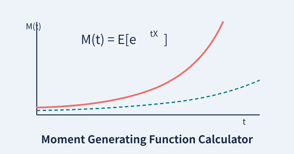
The moment generating function (MGF) of a random variable X is the function M(t) = E[e^(tX)], the expected value of e raised to the power tX. It looks abstract, but it earns its name beautifully: differentiate it once and evaluate at t = 0 and you get the mean E[X]; differentiate it twice and you get E[X²], from which the variance follows at once. Every moment of the distribution is hidden inside this one function, waiting to be extracted by calculus, which is why probability courses treat the MGF as a central tool.
The MGF has a second superpower: uniqueness. If two random variables share the same MGF on an interval around zero, they have the same distribution. That makes the MGF a fingerprint. It is also the easiest way to handle sums: the MGF of a sum of independent variables is simply the product of their MGFs, which is how many textbook results, including the fact that sums of independent Poissons are Poisson, are proved in two lines.
How to Use the MGF Calculator
- Pick a distribution. Choose Binomial, Poisson, Normal, Exponential, Geometric or Uniform from the menu. The parameter fields rename themselves to match.
- Set the parameters. Enter values such as n and p for the binomial, lambda for the Poisson, or mu and sigma for the normal.
- Choose t. Any real value works for most distributions; the exponential and geometric MGFs only exist below a limit, and the calculator tells you when your t falls outside the domain.
- Read the results. You get the symbolic MGF, the MGF with your numbers substituted, M′(0) and M′′(0), the mean, the variance, and the numeric value M(t).
The Six Distributions and Their MGFs
Binomial: M(t) = (1 − p + p·e^t)^n
A binomial variable counts successes in n independent trials with success probability p. Its MGF is the single-trial Bernoulli MGF raised to the power n, a direct consequence of the product rule for sums of independent variables. Differentiating gives E[X] = np and Var(X) = np(1 − p).
Poisson: M(t) = exp( λ (e^t − 1) )
The Poisson distribution counts events in a fixed interval at rate λ. Its MGF is famously tidy, and differentiating at zero shows the mean and variance are both exactly λ, the signature property of the Poisson family. As a check: with λ = 3 and t = 0.1, M(t) = exp(3 × (e^0.1 − 1)) ≈ 1.370962.
Normal: M(t) = exp( μ t + σ² t² / 2 )
For a normal variable with mean μ and standard deviation σ, the MGF is an exponential of a quadratic. The linear term produces the mean μ and the quadratic term produces the variance σ², which is why the normal family is described completely by those two numbers.
Exponential: M(t) = λ / (λ − t), for t below λ
The exponential distribution models waiting times at rate λ. Its MGF is a simple fraction, but it only exists for t below λ, a first taste of the fact that MGFs can have restricted domains. The mean is 1/λ and the variance is 1/λ².
Geometric: M(t) = p·e^t / (1 − (1 − p)·e^t)
This calculator uses the trials convention: X is the number of trials up to and including the first success, taking values 1, 2, 3 and so on. (Some books count the failures before the first success instead, which shifts the mean by one; always check which convention a source uses.) Here E[X] = 1/p and Var(X) = (1 − p)/p², and the MGF exists for t below −ln(1 − p).
Uniform: M(t) = (e^(tb) − e^(ta)) / ( t (b − a) )
For a continuous uniform variable on [a, b] the MGF is a ratio of exponentials, with M(0) = 1 by continuity. The mean is the midpoint (a + b)/2 and the variance is (b − a)²/12.
Why the Derivatives Give the Moments
Expand e^(tX) as a power series and take expectations term by term: M(t) = 1 + t·E[X] + t²/2 · E[X²] + t³/6 · E[X³] and so on. The coefficient of each power of t is a moment divided by a factorial, so differentiating strips away one power at a time and setting t = 0 isolates a single moment. That is why the table in this calculator shows M′(0) beside E[X] and M′′(0) beside E[X²]: they are not two methods that happen to agree, they are the same numbers by construction. Variance then follows from Var(X) = E[X²] − (E[X])², which the calculator also displays.
Students practising these calculations by hand often collect their worked values as data sets, and teachers setting that practice find it easier to keep classes and problem groups organised with a clear plan, for example the room layouts from our Seating Chart Generator when group work is involved.
Common Mistakes to Avoid
- Ignoring the domain. An MGF value at a t where the function does not exist is meaningless. The exponential MGF at t equal to λ divides by zero; the formula has a pole there, not a value.
- Mixing up the geometric conventions. Trials-until-success and failures-before-success differ by exactly 1 in the mean and have different MGFs. State your convention, as this page does.
- Using sigma squared where sigma belongs. The normal MGF is written with σ², but the parameter you type in most calculators, including this one, is σ itself. The calculator squares it for you and shows the substituted formula so you can check.
- Expecting M(t) to be a probability. M(t) is an expected value of an exponential, not a probability; it is 1 at t = 0 and usually grows away from it. Values above 1 are normal.
Where MGFs Earn Their Keep
The MGF is not just an exam ritual. Actuaries use it to price risk: the total claim on a portfolio is a sum of independent individual claims, and because MGFs of sums multiply, the distribution of the total, and therefore its mean and variance, falls out of one product. Queueing theorists use the same trick for waiting times built from exponential pieces, and engineers use it for systems whose total lifetime is a sum of component lifetimes.
Games are full of hidden MGFs. Every dice pool in a tabletop game is a sum of independent rolls, so its damage distribution is a product of simple MGFs; the character statistics produced by tools like our Random Character Generator obey exactly the mathematics on this page. Monte Carlo programmers meet the MGF from the other direction: if you can sample from a distribution, you can estimate its MGF numerically, and scheduling those simulation runs fairly across a term is easier with a plan such as the dates picked by our Random Date Generator.
Most importantly for students, the MGF is the bridge between formulas and understanding. Once you see that the mean and variance are simply the first two derivatives of one function at zero, the zoo of distribution formulas collapses into a single idea with six costumes, and exam questions about unfamiliar distributions stop being frightening: write down the MGF, differentiate, and read off the answer.
Frequently Asked Questions
What does MGF stand for and what is it used for?
MGF stands for moment generating function, M(t) = E[e^(tX)]. It is used to find the mean, variance and higher moments of a distribution by differentiation, to identify distributions, and to derive the distribution of sums of independent random variables.
How do you get the mean and variance from an MGF?
Differentiate once and set t = 0 to get E[X] = M′(0). Differentiate twice to get E[X²] = M′′(0). The variance is then Var(X) = M′′(0) − (M′(0))². This calculator performs all three steps for six standard distributions.
What is the MGF of a Poisson distribution?
For a Poisson variable with rate λ, M(t) = exp( λ (e^t − 1) ). For example, with λ = 3 and t = 0.1 the value is about 1.370962, and the mean and variance are both 3.
Why is M(0) always equal to 1?
Because M(0) = E[e^0] = E[1] = 1 for every distribution. It is a quick sanity check: any claimed MGF that does not equal 1 at t = 0 is wrong.
Does every distribution have an MGF?
No. Heavy-tailed distributions such as the Cauchy have no MGF on any interval around zero, because the expectation of e^(tX) diverges. All six distributions in this calculator have MGFs, though the exponential and geometric ones only exist for t below a stated limit.
Which geometric distribution does this calculator use?
The trials convention: X counts the trials up to and including the first success, so X takes values 1, 2, 3 and so on, with mean 1/p. If your course counts failures before the first success, subtract 1 from the mean and use the same variance.
Is this MGF calculator free?
Yes. It is free, requires no sign-up, and runs entirely in your browser.